
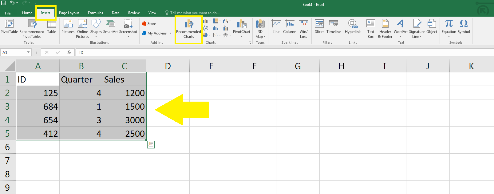
1). Highlight the cells with numerical data that you want to be included in the chart and go to Insert > Recommended Charts.
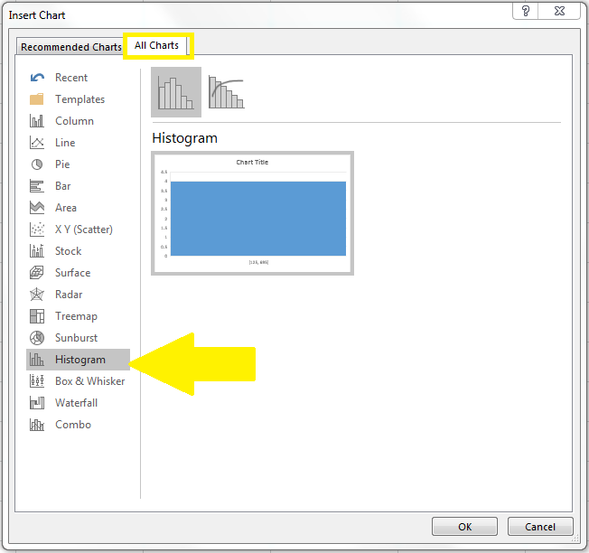
2). Select All Charts > Histogram > OK.
3). Now you have your Histogram Chart.
For a visual of these steps to create a Histogram in Excel, see below.
1. Highlight the cells with numerical data that you want to be included in the chart and go to Insert > Recommended Charts.
2. Select All Charts > Histogram > OK.
3. Your histogram chart will appear directly on your Excel spreadsheet. Use the  and
and  buttons to edit chart elements and design.
